Copulas
A popular approach taken by financial analysts to reduce monetary risk is known as portfolio diversification. In finance, a collection of assets is commonly referred to as a portfolio and is a standard strategy taken by analysts to raise the likelihood of a profitable strategy. Unlike investing in a single asset, portfolios allow for an investor to distribute their resources in an attempt to diversify their approach. Hence, selecting the individual assets to comprise the portfolio is often referred to as portfolio diversification and is an extremely important process with many considerations to account for. In this article, we will be discussing the simple case of a two stock portfolio. More specifically, in order to capitalize on new information as it is acquired, we will be using a pairs-trading approach to manage the portfolio.
In pairs-trading, the investor monitors the movement of two assets—in our case stocks—in relation to one another and uses this information to make decisions on how their portfolio's resources are allocated (Rad et al. 2016). The investor could use this information to re-weight their portfolio by selling shares, buying shares, holding shares, or any combination of the three applied to the two stocks of interest.
In order for pairs-trading to be effective the analyst needs an accurate measure of the historical dependence between stocks, and correlation falls short. In this scenario, the analyst needs a measure of dependence that can describe the significance of new observations and how characteristic or uncharacteristic these observations are considering historical behavior. Simple correlation measures such as Pearson's coefficient and Kendall's tau still play a role in the selection of stocks, but cannot compare to copulas as a dependence measure in this context (Liew and Wu 2013). While copulas remain a somewhat dated (and perhaps controversial) tool, they provide the financial analyst with enough detail about the historical dependence between two stocks to inform judgments about new observations and guide the investment process. Unfortunately, analysts and statisticians alike will always find themselves wanting more data to test their strategies and develop new models. Here we discuss a solution for simulating stock market data for this purpose.
Background
Copulas
As the word copula, from the Latin, roughly means "that which binds" (noa 2021). Thus, the connection between the joint distribution and the marginal distributions is the copula. It is often said that the joint distribution can be fully reconstructed from the copula and marginal distributions. In its purest form, a copula is simply a joint distribution with uniform marginals.
Sklar's Theorem
Any multivariate joint distribution can be written in terms of univariate marginal distribution functions and a copula which describes the dependence structure between the variables.
Consider a \( k \)-dimensional dataset, \( D \), for which we would like to separate into its constituent components: \( k \) univariate marginals and a \( k \)-dimensional copula. Sklar's Theorem allows us to express this \( k \)-dimensional copula as follows:
Let \( (X_1, X_2, \ldots, X_k) \) be some joint multivariate distribution with CDF \( F(\cdot) \) where each random variable \( X_i \) has corresponding CDF \( F_i(\cdot) \). Then, from the probability integral transform we have \( U_i = F_i(X_i) \) where \( U_i \sim \text{Uniform} \). Finally, we can derive the copula,
\[ \begin{align*} F(X_1, X_2, \ldots, X_k) &= P(X_1 \le x_1 \cap X_2 \le x_2 \ldots \cap X_k \le x_k) \\ &= P(F_1^{-1}(U_1) \leq x_1 \cap F_2^{-1}(U_2) \leq x_2 \ldots \cap F_k^{-1}(U_k) \leq x_k) \\ &= P(U_1 \le u_1 \cap U_2 \le u_2 \ldots \cap U_k \le u_k) \\ &= C(U_1, U_2, \ldots, U_k) \end{align*} \]
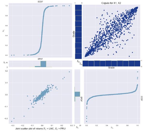
Figure 1: Joint distribution of returns, empirical PDF and CDF of returns, and corresponding empirical copula of returns for the LNC, PRU stocks. Dataset contains about 1000 obs from 2017-01-04 to 2020-12-31.
Gaussian Copula
In the financial context, it would likely prove beneficial to consider both Gaussian copulas as well as the Archimedian class which include the Frank, Gumbel, Clayton, and Joe copulas among others (Nelsen 2006). Due to time constraints, this discussion will be covering one of the simplest of these: the Gaussian Copula. While the Gaussian Copula might not be the optimal choice for financial applications, (the Gaussian copula is somewhat controversial regarding its potential involvement in the 2008 financial crisis as discussed in (Watts 2016)) its simple structure makes it an attractive choice for academic research.
That being said, we will nonetheless refrain from assuming the marginals to be normally distributed and instead follow the process of computing empirical CDFs. The reason we will follow this process is to allow for the proposed algorithm to remain extensible to other copulas and marginal distributions. We emphasize this point because when we later propose a simulation algorithm, we will outline a general solution rather than simply generating correlated normal marginal distributions. Furthermore, we gain the advantage of showing how dependence structure between non-normal marginals can be appropriately modeled with a Gaussian Copula. At any rate, we define the Gaussian Copula as follows:
Given a correlation matrix \( R \in [-1,1]^{d \times d} \) the Gaussian Copula, parameterized by \( R \) is given by,
\[ C_{R}^{\text{Gauss}}(u) = \Phi_{R}(\Phi^{-1}(u_{1}), \ldots, \Phi^{-1}(u_{d})) \]
where \( \Phi_{R} \) is the joint normal CDF and \( \Phi^{-1} \) is the inverse CDF of a normal distribution.
The density is then given by,
\[ c_{R}^{\text{Gauss}}(u) = \frac{1}{\sqrt{\det R}} \exp \left(-\frac{1}{2} \begin{bmatrix} \Phi^{-1}(u_{1}) \\ \vdots \\ \Phi^{-1}(u_{d}) \end{bmatrix}^{T} \cdot (R^{-1} - I) \cdot \begin{bmatrix} \Phi^{-1}(u_{1}) \\ \vdots \\ \Phi^{-1}(u_{d}) \end{bmatrix}\right) \]
c.f. (Arbenz 2013) and (noa 2021) for more details on derivation and (Chen and Fan 2006) for more on the Gaussian copula.
In the bivariate case with the Gaussian copula, with \( \theta \) as the correlation between univariate vectors \( (u, v) \), we notice that \( R \) takes the form
\[ R = \begin{bmatrix} 1 & \theta \\ \theta & 1 \end{bmatrix} \].
Thus, let's consider simplifying the notation for the density function as follows,
\[ C_\theta(u, v) \]
Next, note that as with any joint CDF, the partial derivatives yield conditional distributions.
\[ C_\theta(u\ |\ v) = \frac{\partial C_\theta(u, v)}{\partial u} \]
Pairs-Trading with Copulas
The copula pairs-trading strategy is similar to mean-reversion approaches in that we rely on the assumption that we expect the pair of stocks to revert to their historic relationship at some point in the future. Oftentimes quantitative analysts will refer to this future date as the horizon or investment-horizon. This is similar to the mean-reversion perspective where one might expect a random process to eventually revert to its mean value. The key difference between these approaches is that the pairs-trading approach relies on the historical dependence between two processes rather than the mean of a single process.
Using Sklar's Theorem, we can derive the dependence structure between two variables using the empirical CDFs to create uniform variables, and examining the joint distribution of these uniform random variables, thus constructing the distribution's empirical copula (note that we need only the CDFs to accomplish this). In a financial context, the empirical copula can be constructed from stock returns and fitting a formal analytical copula function to the data becomes possible. This process would proceed with the following steps:
- Let \( R_1 = (r_1^{(1)}, r_1^{(2)}, \dots, r_1^{(t)}) \), \( R_2 = (r_2^{(1)}, r_2^{(2)}, \dots, r_2^{(t)}) \) be the returns of two stocks up to time \( t \).
- Calculate the empirical CDFs \( F_{R_1}(\cdot) \), \( F_{R_2}(\cdot) \).
- Calculate \( U_1 = F_{R_1}(R_1) \), \( U_2 = F_{R_2}(R_2) \).
- Then the empirical copula observations become \( (U_1, U_2) \).
- Fit a copula density function \( C_\theta(R_1, R_2) \) with MLE (or similar) to the observed data \( (U_1, U_2) \) where \( \theta \) is some shape parameter.(Arbenz 2013)
Finally, we are ready to define our pairs-trading strategy:
- With fitted copula density function \( C_\theta (R_1, R_2) \) obtain conditional distributions \[ C_\theta(R_1\ |\ R_2) = \frac{\partial C_\theta(R_1,R_2)}{\partial R_1},\ C_\theta(R_2\ |\ R_1) = \frac{\partial C_\theta(R_1,R_2)}{\partial R_2} \]
- Observe new returns pair at time \( t+1 \): \( (r_1^{(t+1)}, r_2^{(t+1)}) \)
- Evaluate \( C_\theta(r_1^{(t+1)} | r_2^{(t+1)}) \) and \( C_\theta(r_2^{(t+1)} | r_1^{(t+1)}) \)
- Generate trade signal according to some threshold \( K \in (0,1) \):
- If \( C_\theta(r_1^{(t+1)} | r_2^{(t+1)}) > K \) and \( C_\theta(r_2^{(t+1)} | r_1^{(t+1)}) < 1-K \)
- Stock corresponding to \( R_1 \) is overvalued at time \( t+1 \)
- Stock corresponding to \( R_2 \) is undervalued at time \( t+1 \)
Sell stock corresponding to \( R_1 \), buy stock corresponding to \( R_2 \)
- If \( C_\theta(r_2^{(t+1)} | r_1^{(t+1)}) > K \) and \( C_\theta(r_1^{(t+1)} | r_2^{(t+1)}) < 1-K \)
- Stock corresponding to \( R_2 \) is overvalued at time \( t+1 \)
- Stock corresponding to \( R_1 \) is undervalued at time \( t+1 \)
Sell stock corresponding to \( R_2 \), buy stock corresponding to \( R_1 \)
- Else, hold positions.
- If \( C_\theta(r_1^{(t+1)} | r_2^{(t+1)}) > K \) and \( C_\theta(r_2^{(t+1)} | r_1^{(t+1)}) < 1-K \)
Note: This approach is functionally equivalent to the process outlined in (Botha et al. 2013).
Fortunately, for the Gaussian copula we can take advantage of the symmetric structure and only calculate one conditional since \( C_\theta(u | v)=C_\theta(v | u) \) and this simplifies steps 1 and 4. Furthermore, since in the case of the Gaussian copula our shape parameter is the correlation coefficient \( \theta \) we do not need to use MLE to fit the density function (while this hardly makes a difference, it is worth noting).
Example
Let's develop some intuition on how this process works. Looking at Figure 1 we see that we have completed the 5 step process of transforming observations to arrive at an empirical copula, and fitting a Gaussian copula density function to the data. Now, it is time to make a trade-decision...
At time \( t+1 \), we observe the point highlighted in red. First, notice that this point lies quite far from where we might expect it to land.
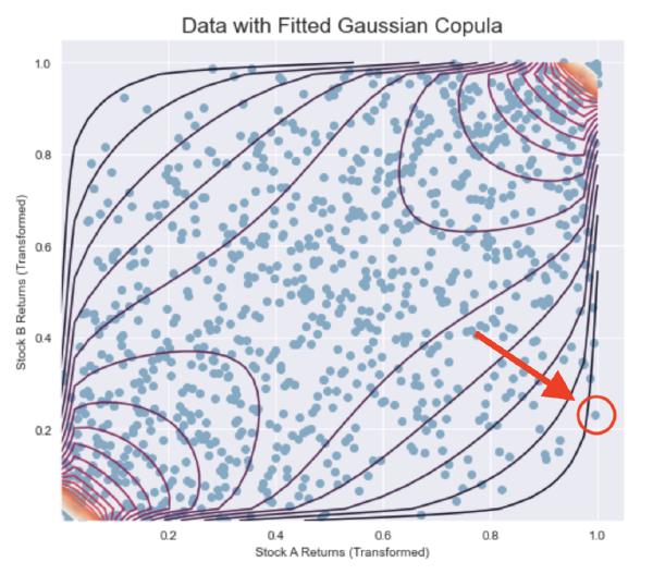
From Figure 2 we can see that depending on what perspective we choose to take, the point should either lie closer to the southwest quadrant or the northeast quadrant.
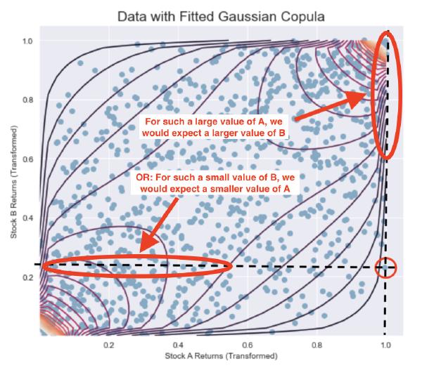
The two points of view can represent the two perspectives of \( C_\theta(r_A^{(t+1)} | r_B^{(t+1)}) \) and \( C_\theta(r_B^{(t+1)} | r_A^{(t+1)}) \) alluded to earlier.
Similar to how we evaluated the conditional values in the mathematically outlined procedure to make a trade decision, we can use our graphical intuition to achieve the same result:
- Given \( r_B^{(t+1)} \), Stock A is overvalued
We expect Stock A to fall in price
- Given \( r_A^{(t+1)} \), Stock B is undervalued
We expect Stock B to rise in price
Buy Stock B, sell Stock A
As alluded to earlier, these figures also illustrate how the copula can act as a proxy for risk quantification for the financial analyst. As the points move away from their expected location, we are more certain that the observations are less consistent with historical behavior. Thus, certainty—and consequently risk—can be quantified by the fitted copula's conditional density functions.
Methods: Data Simulation
In situations where real-world data is limited or an analyst wants to study phenomena there are limited techniques available for simulating data that preserves a desired dependence structure. It therefore seems worthwhile to consider an algorithm that describes how one could randomly simulate data which follows an analytical copula density function. Ideally, the user would be able to specify the desired copula along with the desired marginal distributions and simulate plausible stock prices using the proposed algorithm.
Rosenblatt Transformation
To simulate multivariate data from a specified density function, we first have to consider a multivariate extension of the probability integral transform—the Rosenblatt Transformation—as proposed by Murray Rosenblatt in Remarks on a Multivariate Transformation(Rosenblatt 1952).
Definition (Rosenblatt Transformation)
Let \( X=(X_1, \dots, X_k) \) be a random vector with distribution function \( F(x_1, \dots, x_k) \). Let \( z=(z_1, \dots, z_k)=Tx=T(x_1,\dots, x_k) \), where \( T \) is the transformation considered. Then \( T \) is given by,
\[ \begin{array}{l} z_{1}=P\{X_{1} \leq x_{1}\}=F_{1}(x_{1}) \\ z_{2}=P\{X_{2} \leq x_{2} | X_{1}=x_{1}\}=F_{2}(x_{2} | x_{1}) \\ \vdots \\ z_{k}=P\{X_{k} \leq x_{k} | x_{k-1}=x_{k-1}, \dots, X_{1}=x_{1}\}=F_{k}(x_{k} | x_{k-1}, \dots, x_{1}) \end{array} \]
It can be shown that \( Z=TX \) is then uniformly distributed on the k-dimensional hypercube,
\[ \begin{aligned} P\{Z_{i} \leq & z_{i} ; i=1, \dots, k\} \\ &=\int_{\{Z | z_{i} \leq z_{i}\}} \dots \int d_{x_{k}} F_{k}(x_{k} | x_{k-1}, \dots, x_{1}) \dots d_{x_{1}} F_{1}(x_{1}) \\ &=\int_{0}^{z_{k}} \dots \int_{0}^{z_{1}} d z_{1} \dots d z_{k}=\prod_{i=1}^{k} z_{i} \end{aligned} \]
when \( 0 \leq z_i \leq 1, i=1,\dots,k \). Therefore, \( Z_1,\dots,Z_k \) are uniformly and independently distributed on \( [0,1] \)
c.f. [6] for more details
Rosenblatt Transformation - Normal Case
Let's restrict our problem space to only the case of the multivariate normal distribution. As discussed in (Pumi and Lopez 2010) and (Nelsen 2006), when \( F(x_1,\dots,x_k) \) is a normal distribution with mean \( M=(m_1,\dots,m_k) \) and covariance matrix \( \Lambda^{(r)}={\lambda_{ij}},\ i,j = 1,\dots,r \le k \), and \( \Lambda_{ij}^{(r)} \) be the co-factor of \( {\lambda_{ij}} \) in \( \Lambda^{(r)} \). The transformation \( T \) is then given by,
\[ \begin{aligned} F_{1}(x_{1}) &=\Phi\left(\frac{x_{1}-m_{1}}{\sqrt{\lambda_{11}}}\right) \\ F_{2}(x_{2} | x_{1}) &=\Phi\left(\frac{x_{2}-m_{2}+(\Lambda_{21}^{(2)} / \Lambda_{22}^{(2)})(x_{1}-m_{1})}{\sqrt{\Lambda^{(2)} / \Lambda_{22}^{(2)}}}\right), \\ \vdots & \\ F_{k}(x_{k} | x_{k-1}, \dots, x_{1}) &=\Phi\left(\frac{x_{k}-m_{k}+\sum_{j=1}^{k-1}(\Lambda_{k j} / \Lambda_{k k})(x_{j}-m_{j})}{\sqrt{\Lambda / \Lambda_{k}}}\right) . \end{aligned} \]
Considering the bivariate case, let \( F(x_1, x_2) \) be a normal distribution with means \( m_1, m_2 \), variances \( \sigma_1, \sigma_2 \), and correlation coefficient \( \rho \). With \( \Phi(\cdot) \) as the normal CDF, the transformation is then,
\[ \begin{aligned} F_{1}(x_{1}) &=\Phi\left(\frac{x_{1}-m_{1}}{\sigma_{1}}\right) \\ F_{2}(x_{2} | x_{1}) &=\Phi\left(\frac{x_{2}-m_{2}+\frac{\rho \sigma_{1}}{\sigma_{2}}(x_{1}-m_{1})}{\sigma_{2} \sqrt{1-\rho^{2}}}\right) . \end{aligned} \]
Copula Data Simulation: Algorithm 1
As the probability integral transform is inverted to arrive at the inverse sampling procedure, we propose a similar approach to arrive at the Inverse Rosenblatt Transformation.
Inverse Rosenblatt Transformation (Normal Case)
Considering the bivariate case, let \( U_1, U_2 \sim Uniform \). Designate our target joint distribution \( F(x_1, x_2) \) to be a normal distribution with means \( m_1, m_2 \), variances \( \sigma_1, \sigma_2 \), and correlation coefficient \( \rho \). With \( \Phi^{-1}(\cdot) \) as the normal quantile function, the transformation is then,
\[ \begin{aligned} x_1 &= \Phi^{-1}(U_1)\sigma_{1}+m_1 \\ x_2 &= \Phi^{-1}(U_2)(\sigma_2 \sqrt{1-\rho^2})+m_2-\frac{\rho\sigma_1}{\sigma_2}(x_1-m_1) \end{aligned} \]
For this case, we consider the following process:
- Simulate \( U_1, U_2 \sim Uniform(0,1) \).
- Let \( x_1 = \Phi^{-1}(U_1)\sigma_{1}+m_1 \).
- Let \( x_2 = \Phi^{-1}(U_2)(\sigma_2 \sqrt{1-\rho^2})+m_2-\frac{\rho\sigma_1}{\sigma_2}(x_1-m_1) \).
- The desired sample is \( (x_1,x_2) \) and follows a multivariate normal distribution such that \( x_1\sim N(m_1, \sigma_1) \), \( x_2\sim N(m_2, \sigma_2) \) with \( Corr[x_1, x_2]=\rho \).
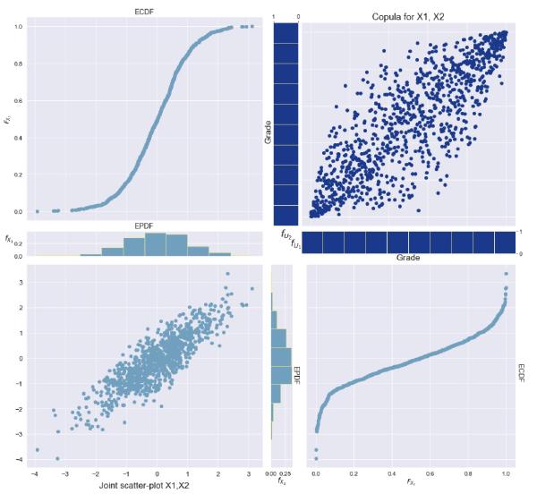
Sample data simulated with this process, along with its copula, can be seen in Figure 3 below.
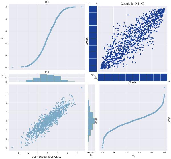
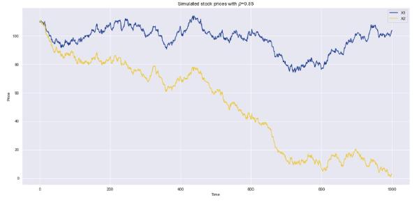
Since these results strongly resemble the results from the first proposed algorithm, let's demonstrate the flexibility of our proposed algorithm. To do this, we simulate data just as before but instead specify one of our marginal distributions to follow a different normal distribution: \( N(-0.1, 1) \). Notice in the figures below that the returns of the affected stock will cause its price to decrease, and the stock prices will hardly look correlated. However, recall that it is in fact the stock returns that are correlated rather than the prices themselves.
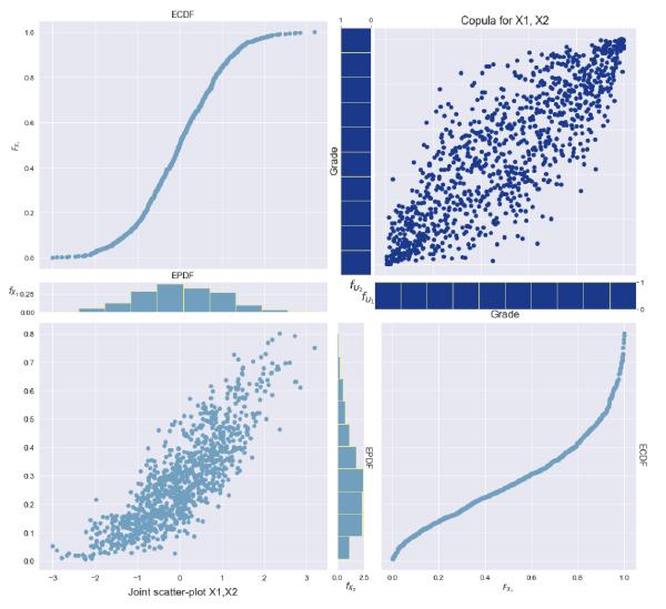
Finally, to emphasize our ability to control the marginal distributions, we will set one of the marginals to follow a \( Beta(2,5) \) distribution and observe the same copula.
Conclusion
In conclusion, we have shown a method for simulating univariate time series data suitable for pairs-trading models. Strengths of our approach include the ability to choose a copula density function and the ability to specify any marginal distribution while maintaining the copula dependence structure. Our hope is that this material could benefit future work in the topic of copula-based algorithmic trading. Opportunities for future work include:
- Stress-testing copula models with noisy data, to determine how robust copula strategies are to noise.
- Evaluating how sensitive copula models are to assets with low liquidity (market slippage).
- Investigating whether copulas can help optimize the aggressiveness of a strategy by being a proxy for risk.
References
- (2021). Copula (probability theory). Page Version ID: 1021423478.
- Arbenz, P. (2013). Bayesian Copulae Distributions, with Application to Operational Risk Management—Some Comments. Methodology and Computing in Applied Probability, 15(1):105–108.
- Botha, I., Stander, Y., and Marais, D. (2013). Trading strategies with copulas. Journal of Economic and Financial Sciences, 6:103–126.
- Chen, X. and Fan, Y. (2006). Estimation of copula-based semiparametric time series models. Journal of Econometrics, 130(2):307–335.
- Liew, R. Q. and Wu, Y. (2013). Pairs trading: A copula approach. Journal of Derivatives & Hedge Funds, 19(1):12–30.
- Murray Rosenblatt (1952). Remarks on a Multivariate Transformation. The Annals of Mathematical Statistics, 23(3):470–472.
- Nelsen, R. B. (2006). An Introduction to Copulas. Springer Series in Statistics. Springer-Verlag, New York, 2 edition.
- Pumi, G. and Lopes, S. R. C. (2010). Simulation of Univariate Time Series Using Copulas. page 6.
- Rad, H., Low, R. K. Y., and Faff, R. (2016). The profitability of pairs trading strategies: distance, cointegration and copula methods. Quantitative Finance, 16(10):1541–1558. Publisher: Routledge _eprint: https://doi.org/10.1080/14697688.2016.1164337.
- Watts, S. (2016). The Gaussian Copula and the Financial Crisis: A Recipe for Disaster or Cooking the Books? page 25.